Working with STAC

What is a STAC Catalog?

STAC stands for SpatioTemporal Asset Catalog. It is a common language to describe geospatial information, so it can be more easily worked with, indexed, and discovered. Spatial information is stored in a geoJSON format, which can be easily adapted to different domains. The goal of STAC is to enable a global index of all imagery derived data products with an easily implementable standard for organization to expose their data in a persistent and reliable way. STAC objects are hosted in geoJSON format as HTML pages.

GEO BON STAC Catalog

Pipelines can be created using layers pulled from any STAC catalog, such as the Planetary Computer. GEO BON hosts a STAC catalog that contains many commonly used data layers, which can be explored in JSON format or in a more user-friendly viewer.

There is a step to pull and filter data from a STAC catalog in BON in a Box called ‘Load from STAC’, where users can specify the layers, bounding box, projection system, and spatial resolution they are interested in. It outputs a geoJSON file that becomes an input into a subsequent pipeline step.

Working with the STAC Catalog in R

Data in STAC catalogs can be loaded directly into R and visualized using the rstac package.

To start, install and load the following packages.

library(gdalcubes)
library(rstac)
library(knitr)
library(stars)

Loading required package: abind

Loading required package: sf

Linking to GEOS 3.12.1, GDAL 3.8.4, PROJ 9.3.1; sf_use_s2() is TRUE

Next, connect to the STAC catalog using the stac function in the rstac package.

stac_obj <- stac("https://stac.geobon.org/")

In the STAC catalog, layers are organized into collections. To make a list of the collections:

collections <- stac_obj |> collections() |> get_request()

And to view the collections and their descriptions in a table.

df<-data.frame(id=character(),title=character(),description=character())
for (c in collections[['collections']]){
  df<-rbind(df,data.frame(id=c$id,title=c$title,description=c$description))
}
kable(head(df))

id	title	description
chelsa-clim	CHELSA Climatologies	CHELSA Climatologies
gfw-lossyear	Global Forest Watch - Loss year	Global Forest Watch - Loss year
soilgrids	Soil Grids datasets	SoilGrids aggregated datasets at 1km resolution
ghmts	Global Human Modification of Terrestrial Systems	The Global Human Modification of Terrestrial Systems data set provides a cumulative measure of the human modification of terrestrial lands across the globe at a 1-km resolution. It is a continuous 0-1 metric that reflects the proportion of a landscape modified, based on modeling the physical extents of 13 anthropogenic stressors and their estimated impacts using spatially-explicit global data sets with a median year of 2016.
gfw-treecover2000	Global Forest Watch - Tree cover 2000	Global Forest Watch - Tree cover 2000
gfw-gain	Global Forest Watch - Gain	Global Forest Watch - Gain

To search for a specific collection. Here we will search for the land cover collection from EarthEnv.

it_obj <- stac_obj |>
  stac_search(collections = "earthenv_landcover") |>
  post_request() |> items_fetch()
it_obj

###Items
- features (12 item(s)):
  - class_9
  - class_8
  - class_7
  - class_6
  - class_5
  - class_4
  - class_3
  - class_2
  - class_12
  - class_11
  - class_10
  - class_1
- assets: data
- item's fields: 
assets, bbox, collection, geometry, id, links, properties, stac_extensions, stac_version, type

View the available layers in this collection.

it_obj <- stac_obj |>
  collections("earthenv_landcover") |> items() |>
  get_request() |> items_fetch()
it_obj

###Items
- features (12 item(s)):
  - class_9
  - class_8
  - class_7
  - class_6
  - class_5
  - class_4
  - class_3
  - class_2
  - class_12
  - class_11
  - class_10
  - class_1
- assets: data
- item's fields: 
assets, bbox, collection, geometry, id, links, properties, stac_extensions, stac_version, type

View the properties of the first item (layer).

it_obj[['features']][[1]]$properties

$class
[1] "9"

$datetime
[1] "2000-01-01T00:00:00Z"

$`proj:epsg`
[1] 4326

$description
[1] "Urban/Built-up"

$full_filename
[1] "consensus_full_class_9.tif"

We can summarize each layer in a table

df<-data.frame(id=character(),datetime=character(), description=character())
for (f in it_obj[['features']]){
  df<-rbind(df,data.frame(id=f$id,datetime=f$properties$datetime,description=f$properties$description))
}
kable(head(df))

id	datetime	description
class_9	2000-01-01T00:00:00Z	Urban/Built-up
class_8	2000-01-01T00:00:00Z	Regularly Flooded Vegetation
class_7	2000-01-01T00:00:00Z	Cultivated and Managed Vegetation
class_6	2000-01-01T00:00:00Z	Herbaceous Vegetation
class_5	2000-01-01T00:00:00Z	Shrubs
class_4	2000-01-01T00:00:00Z	Mixed/Other Trees

Now, you can load one of the items with the stars package, which allows access to files remotely in a fast and efficient way by only loading the areas that you need.

Here we will select the layer representing the percentage of “Evergreen/Deciduous Needleleaf Trees”, which is the 12th layer in the collection.

lc1<-read_stars(paste0('/vsicurl/',it_obj[['features']][[12]]$assets$data$href), proxy = TRUE)
plot(lc1)

downsample set to 23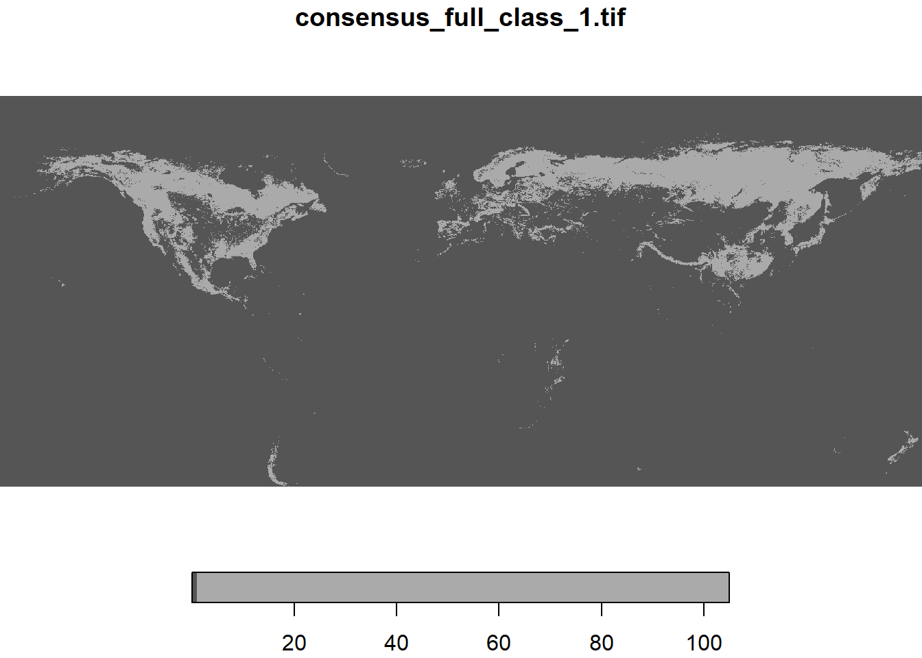

You can crop the raster by a bounding box and visualize it.

bbox<-st_bbox(c(xmin = -76, xmax = -70, ymax = 54, ymin = 50), crs = st_crs(4326))
lc2 <- lc1 |> st_crop(bbox)

pal <- colorRampPalette(c("black","darkblue","red","yellow","white"))
plot(lc2,breaks=seq(0,100,10),col=pal(10))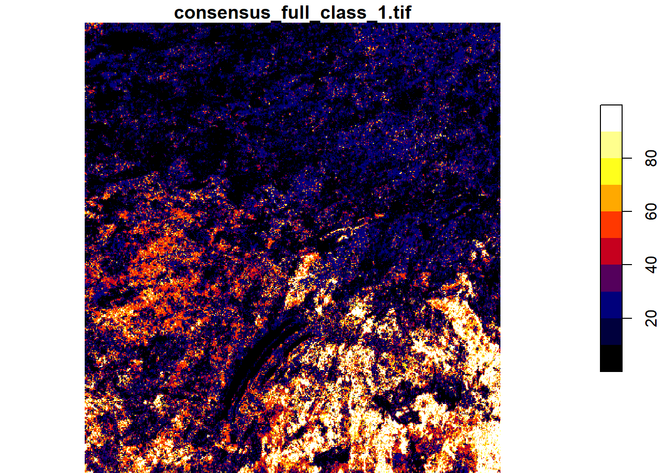

You can now save this object to your computer in Cloud Optimized GeoTiff (COG) format. COG works on the cloud and allows the user to access just the part of the file that is needed because all relevant information is stored together in each tile.

# Replace " ~ " for the directory of your choice on your computer.
write_stars(lc2,'~/lc2.tif',driver='COG',options=c('COMPRESS=DEFLATE'))

Note that for a layer with categorical variables, saving is more complex.

lc1 |> st_crop(bbox) |> write_stars('~/lc1.tif', driver='COG', RasterIO=c('resampling'='mode'),
options=c('COMPRESS=DEFLATE', 'OVERVIEW_RESAMPLING=MODE', 'LEVEL=6',
'OVERVIEW_COUNT=8', 'RESAMPLING=MODE', 'WARP_RESAMPLING=MODE', 'OVERVIEWS=IGNORE_EXISTING'))

Working with GDAL Cubes

The R package gdalcubes allows for the processing of four dimensional regular raster data cubes from irregular image collections, hiding complexities in the data such as different map projections and spatial overlaps of images or different spatial resolutions of spectral bands. This can be useful for working with many layers or time series of satellite imagery.

The following step is necessary for GDAL Cubes to work with STAC catalog data.

for (i in 1:length(it_obj$features)){
  it_obj$features[[i]]$assets$data$roles='data'
}

You can filter based on item properties and create a collection.

st <- stac_image_collection(it_obj$features, asset_names=c('data'),
             property_filter = function(f){f[['class']] %in% c('1','2','3','4')},srs='EPSG:4326')

Next, you can build a GDAL cube to process or visualize the data. This cube can be in a different CRS and resolution from those of the original elements/files. However, the time dimension must capture the temporal framework of the item. dt is expressed as a time period, P1M is a period of one month, P1Y is a period of one year. Resampling methods should be tailored to the data type. For categorical data, use “mode” or “nearest”. For continuous data, use “bilinear”. Aggregation is relevant only when multiple rasters overlap.

Here is an example that sums the four forest categories using aggregation=“sum”, with a change of the reference system to use Quebec Lambert (EPSG:32198) and a resolution of 1 km.

bbox<-st_bbox(c(xmin = -483695, xmax = -84643, ymin = 112704 , ymax = 684311), crs = st_crs(32198))

v <- cube_view(srs = "EPSG:32198", extent = list(t0 = "2000-01-01", t1 = "2000-01-01", left = bbox$xmin, right =bbox$xmax, top = bbox$ymax, bottom = bbox$ymin),
dx=1000, dy=1000, dt="P1D", aggregation = "sum", resampling = "mean")

Create a raster cube

lc_cube <- raster_cube(st, v)

Save the resulting file to your computer

# Replace " ~ " for the directory of your choice on your computer.
lc_cube |> write_tif('~/',prefix='lc2',creation_options=list('COMPRESS'='DEFLATE'))

Plot the raster cube

lc_cube |> plot(zlim=c(0,100),col=pal(10))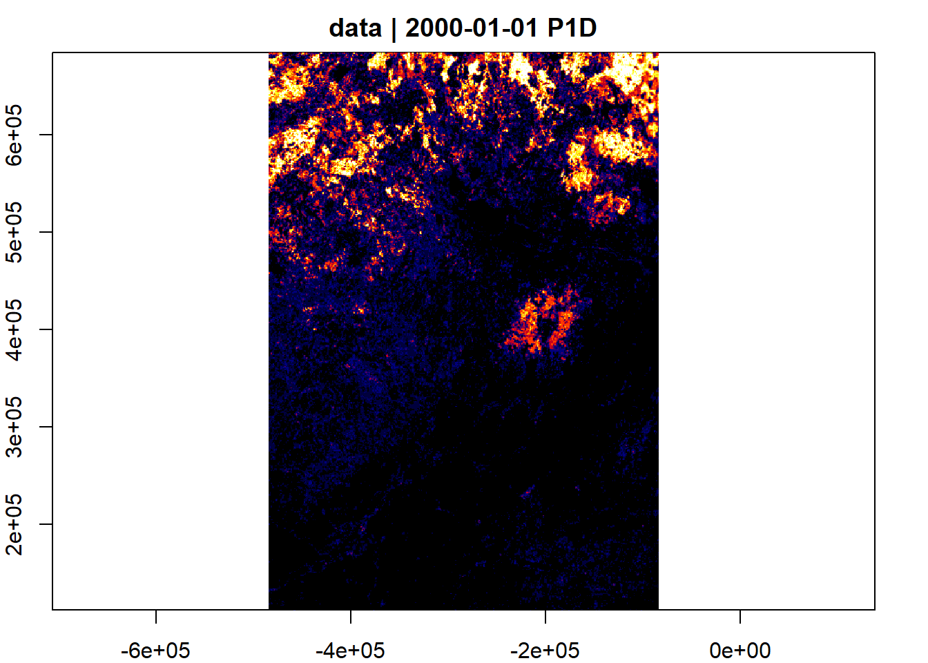

Use the accessibility from cities dataset, keeping the same CRS and extent

it_obj <- stac_obj |>
  collections("accessibility_to_cities") |> items() |>
  get_request() |> items_fetch()
v <- cube_view(srs = "EPSG:32198", extent = list(t0 = "2015-01-01", t1 = "2015-01-01",
                                                left = bbox$xmin, right =bbox$xmax, top = bbox$ymax, bottom = bbox$ymin),
                                                dx=1000, dy=1000, dt="P1D", aggregation

 = "mean", resampling = "bilinear")
for (i in 1:length(it_obj$features)){
  it_obj$features[[i]]$assets$data$roles='data'
}
st <- stac_image_collection(it_obj$features)
lc_cube <- raster_cube(st, v)
lc_cube |> plot(col=heat.colors)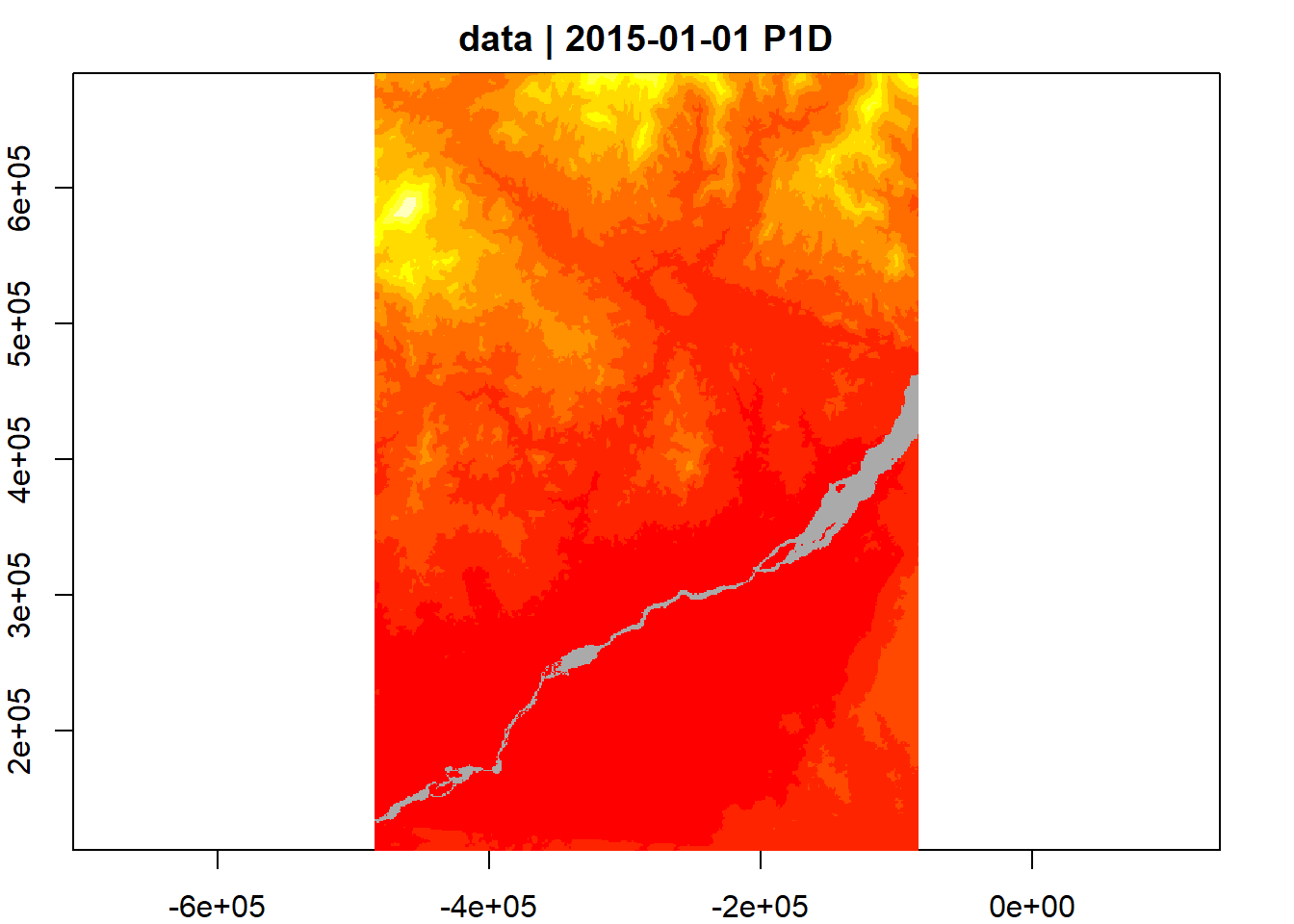

Use the CHELSA dataset on climatologies and create an average map for the months of June, July, and August 2010 to 2019

it_obj <- s_obj |>
  stac_search(collections = "chelsa-monthly", datetime="2010-06-01T00:00:00Z/2019-08-01T00:00:00Z") |>
  get_request() |> items_fetch()

v <- cube_view(srs = "EPSG:32198", extent = list(t0 = "2010-06-01", t1 = "2019-08-31", left = bbox$xmin, right =bbox$xmax, top = bbox$ymax, bottom = bbox$ymin), dx=1000, dy=1000, dt="P10Y", aggregation = "mean",resampling = "bilinear")

for (i in 1:length(it_obj$features)){
  names(it_obj$features[[i]]$assets)='data'
  it_obj$features[[i]]$assets$data$roles='data'
}

anames=unlist(lapply(it_obj$features,function(f){f['id']}))

st <- stac_image_collection(it_obj$features, asset_names = 'data', property_filter = function(f){f[['variable']] == 'tas' & (f[['month']] %in% c(6,7,8)) })

c_cube <- raster_cube(st, v)

c_cube |> plot(col=heat.colors)

c_cube |> write_tif('~/',prefix='chelsa-monthly',creation_options=list('COMPRESS'='DEFLATE'))