Instructions for adapting your code to an analysis pipeline
Analysis pipelines in BON in a Box are workflows that have been adapted to its pipelines framework. Here we will walk you through a few steps to adapt your code to run in BON in a Box.
General GitHub contribution workflow
Contributors will follow the GitHub flow when contributing pipelines to BON in a Box. Contributors can follow these steps:
Make sure you have a personal/institutional GitHub repository.
If BON in a Box developers have granted you access to the repository, create a branch for your pipeline. Otherwise, fork the bon-in-a-box-pipelines repository to your personal GitHub repository and then clone it to your computer.
Create a branch from the main branch for your pipeline, with a descriptive branch name (e.g. ProtConn_pipeline).
Create your pipeline on this branch. Make sure it adheres to the pipeline standards.
When it is complete, create a pull request (instructions here) to the main branch on the bon-in-a-box-pipelines GitHub and fill out the peer review template that will autofill in the pull request, suggesting at least two potential peer reviewers.
When peer review is complete, make any suggested changes to the pipeline and resubmit.
When the pipeline has been accepted, it will be merged to the main branch and published on Zenodo with a DOI.
The BON in a Box team will contact you for any bug fixes or feature requests, and new releases will follow the versioning structure specified at the bottom of this page.
During the development process of the pipeline, regularly merge the main branch to your branch to avoid potential conflicts when merging your branch.
How to write a script video tutorial
How to create a pipeline video tutorial
Analysis workflows can be adapted to BON in a Box pipelines using a few simple steps. Once BON in a Box is installed on your computer, pipelines can be edited and run locally by creating files in your local BON-in-a-box folder cloned from the GitHub repository. Workflows can be written in a variety of languages, including R, Julia, and Python, and not all pipeline steps need to be in the same language.
Before you start
Make sure that you are working in the right environment when running code in BON in a Box. This can be in your code editor of choice, such as Visual Studio Code opened to the BON in a Box pipelines folder cloned to your computer from GitHub, or an R Studio project set up with the BON in a Box GitHub repository. This will make it easier to pull and push to the GitHub repository later.
Step 1: Plan your pipeline
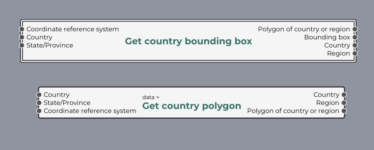
The first step is to sketch out what your pipeline will look like. This includes breaking up your workflow into logical steps that perform one task and could potentially be reused in other pipelines. Think of the inputs and outputs that you want each script to have and how you want to connect these into a full pipeline.
Here is an example:
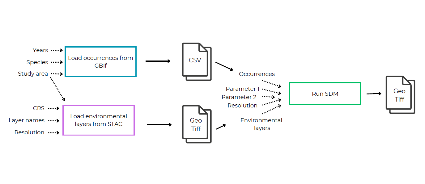
Check if any of the steps you need are already available in BON in a Box to avoid having to rewrite them.
Step 2: Break up your scripts
You can start writing the individual scripts in your pipeline. If you already have an analysis workflow, break this up into individual scripts representing the steps of the pipeline. Plan what you want as the inputs and outputs for each script.
Step 3: Create a YAML file
Each script should be accompanied by a YAML file (.yml extension) that specifies inputs and outputs of that step of the pipeline.
Markdown is supported for pipeline, script, input, and output descriptions. See this CommonMark quick reference for allowed markups. These can include special characters, links, and images.
Name and description
YAML files should begin with a name, description, and the authors of the script. The name should be the name of the script described by the YAML file (script_name.R below). Save the file with the same name as the script that it describes but with a .yml extension (e.g. if the script is called my_script.R the YAML should be called my_script.yml).
Example:
script: script_name.R
name: Script Name
description: Describe what the script does
author:
  - name: John Doe (john.doe@gmail.com)
  - name: Jane Doe (jane.doe@gmail.com)
Inputs
Next, the YAML file should specify the inputs of the script. These inputs will either be outputs from the previous script, which can be connected by lines in the pipeline editor, or specified by the user in the input form.
All input and output ids should follow the snake case naming conventions. Names should be all lowercase with underscores instead of spaces. For example, an input labelled “Species name” would have the snake case id of “species_name”. This id will be the name of the input parameter in your code.
Here is an example where the inputs are a coordinate reference system and a distance, specified by the user:
inputs:
  crs:
    label: coordinate reference system for output
    description: ESPG coordinate reference system for output
    type: text
    example: "EPSG:4326"
  distance:
    label: Distance
    description: Some distance measurement (in meters) for a parameter
    type: int
    example: 1000
Specifying an example will auto-fill that input with the example unless changed by the user. If you do not want an example that auto-fills the input, write “example: null”. This will leave the input blank unless the user adds one. Not specifying any example will cause an error. It is mandatory that a script can be run successfully by leaving all the examples and simply pressing Run.
There are several different types of user inputs that can be specified in the YAML file:
| “Type” attribute in the yaml | UI rendering | Description |
|---|---|---|
| boolean | Plain text | true/false |
| float or float[] (float array) | Plain text | positive or negative numbers with a decimal point, accepts int and a valid input. |
| int or int[] (int array) | Plain text | integer |
| options1 | Dropdown menu | Select one from predefined options |
| options[]1 | Multi-select dropdown menu | Select several from predefined options |
| text or text[] (text array) | Plain text | text input (words) |
| (any unknown type) | Plain text |
- Note that the square brackets specify an array, where the user can input multiple values separated by a comma. This is useful if you want the analysis to run with several different parameters (e.g. for multiple species or with multiple raster bands).
1options type requires an additional options attribute to be added with the available options.
options_example:
  label: Options example
  description: The user has to select between a fixed number of text options. Also called select or enum. The script receives the selected option as text.
  type: options
  options:
  - first option
  - second option
  - third option
  example: third option
The user inputs can also be file types if you want to upload a file or connect the script to a previous one that outputs a specific file type. There are several file types that you can specify:
| File Type | MIME type to use in the yaml | Description |
|---|---|---|
| CSV | text/csv | Comma separated values file format (.csv) |
| GeoJSON | application/geo+json | GeoJSON file format (.geojson) |
| GeoPackage | application/geopackage+sqlite3 | GeoPackage file format (.gpkg) |
| GeoTIFF2 | image/tiff;application=geotiff | GeoTIFF file format (.tif) |
| Shapefile | application/dbf | Shapefile format (.shp) |
| Text | text/plain | Plain text output (no need to save as a format just output in the script) |
| TSV | text/tab-separated-values | Tab separated values format (.tsv) |
For example:
inputs:
  landcover_raster:
    label: Raster of landcover
    description: Landcover data pulled from EarthEnv database with 1x1km resolution
    type: application/geo+json
    example: null
  species_occurences:
    label: Occurence points of species
    description: Occurence points from GBIF or uploaded by the user
    type: text/csv
    example: null
The input type can also be set to a limited number of keywords that will automatically generate standardized selectors adapted for the input type. For example, specifying ‘country’ as input type will create a dropdown menu with a standardized list of countries from GeoNames. Selecting ‘bboxCRS’ will allow the user to define a bounding box from a country or by clicking on a map. Here is the current list of available selectors:
| Input name | Description | |
|---|---|---|
| country | Creates a selector (drop down menu) with a standardized list of countries. GeoNames is used as the reference for the country list. | |
| countryRegion | Creates a selector (drop down menu) with a standardized list of regions (provinces, states, etc) within a selected country. GeoNames is used as the reference for the list of regions. | |
| countryRegionCRS | Creates a selector (drop down menu) for choosing a coordinate reference system adapted for a specific country and/or region. | |
| CRS | Creates a selector for specifying a coordinate reference system. | |
| bboxCRS | Creates a button to open an interface that allows the user to specify a bounding box (geographical minima and maxima) based on an optional selection of country/region and on a CRS, or by clicking on the map to set the bounds of the area of interest for the analysis. |
Note that the use of these selectors will create objects that contain multiple elements. For example, the country selector will create an input object that contains the country name in English, the ISO3 code of the country, the ISO2 code, as well as the bounding box of that country, in longitude, latitude coordinates. See the full list of those keys for each selector here.
Outputs
After specifying the inputs, you can specify the files that you want to output for that script. These can either be final pipeline outputs, outputs for that step to connect to another step, or both.
There are also several types of outputs that can be created
| File Type | MIME type to use in the yaml | UI rendering |
|---|---|---|
| CSV | text/csv | HTML table (partial content) |
| GeoJSON2 | application/geo+json | Map |
| GeoPackage | application/geopackage+sqlite3 | Link |
| GeoTIFF3 | image/tiff;application=geotiff | Map widget (leaflet) |
| HTML | text/html | Open in new tab |
| JPG | image/jpg | tag |
| Shapefile | application/dbf | Link |
| Text | text/plain | Plain text |
| TSV | text/tab-separated-values | HTML table (partial content) |
| (any unknown type) | Plain text or link |
2 GeoJSON coordinates must be in WGS 84. See specification section 4 for details.
3 When used as an output, image/tiff;application=geotiff type allows an additional range attribute to be added with the min and max values that the tiff should hold. This will be used for display purposes.
map:
  label: My map
  description: Some map that shows something
  type: image/tiff;application=geotiff
  range: [0.1, 254]
  example: https://example.com/mytiff.tif
Here is an example output:
outputs:
  result:
    label: Analysis result
    description: The result of the analysis, in CSV form
    type: text/csv
  result_plot:
    label: Result plot
    description: Plot of results
    type: image/png
Specifying R and Python package dependencies with conda
“Conda provides package, dependency, and environment management for any language.” If a script is dependent on a specific package version, conda will load that package version to prevent breaking changes when packages are updated. BON in a Box uses a central conda environment that includes commonly used libraries, and supports dedicated environments for the scripts that need it.
This means that instead of installing packages during script execution scripts, they are installed in the R environment in conda. Note that you still need to load the packages in your scripts using the library() command for R or import for Python.
Check if the libraries you need are in conda
To check if the packages you need are already in the default conda environment, go to runners/conda/r-environment.yml or runners/conda/python-environment.yml in the BON in a Box project folder. The list of packages already installed can be found under “dependencies”.
If all the packages that you need are in the R environment file and you do not need specific package versions, you do not need to specify a conda sub environment and you can skip the next step.
Specify a conda sub-environment in your YML file
If you include a conda section, make sure you list all your dependencies. If you specify a conda environment in your YML file, it is creating a new separate conda environment, not a supplement to the base environment. This means that all of the packages that you need for the script need to be specified here, even if they are in the r-environment.yml file.
Search for your package names on anaconda. Packages that are in anaconda will be recognized by conda and can be included in the conda sub-environment in the YML file. If your package is not there, see below.
Note that every conda sub environment and script in R must load rjson because it is necessary for running the pipelines in BON in a Box
Example of conda sub-environment for an R script:
conda: # Optional: if you script requires specific versions of packages.
  channels:
    - conda-forge # make sure to put conda forge first
    # - r # use this chanel only if some packages are not available in conda-forge
  dependencies:
    - r-rjson # read inputs and save outputs for R scripts
    - r-terra
    - r-ggplot2
    - r-rredlist=1.0.0 # package=version
Example of conda sub-environment for a python script. You do not need to put anything after conda-forge or before the package names when specifying a conda environment for python.
conda:
  channels:
    - conda-forge
  dependencies:
    - openeo
    - pandas
Conda dependency management is not available in Julia. There is a central project at /julia_depot/.
For more information, refer to the conda documentation.
Loading packages that are not available in conda
If you need a package that is not available in conda, such as one downloaded from GitHub, install the package directly in the script. Do not add these packages to the conda portion of the yml file because conda will not be able to recognize them.
In R, concurrent installation of packages can be problematic (for example when running the same script multiple times in parallel). For this language only, you must use the function `biab_ensure_package(…)` that monitors the R locking mechanism to hold back the concurrent scripts during installation. Below is an example usage:
biab_ensure_package(
    "duckdbfs",
    version = "0.1.2",
    installer = function() {
        remotes::install_version("duckdbfs", version = "0.1.2", dependencies = FALSE, upgrade = "never")
    }
)

biab_ensure_package(
    "duckspatial",
    version = "0.9.0",
    installer = function() {
        remotes::install_github("Cidree/duckspatial@v0.9.0", dependencies = FALSE, upgrade = "never")
    }
)

library(duckdbfs)
library(duckspatial)
Examples
Full example of a YAML file:
script: script_name.R
name: Script Name
description: Describe what the script does
author:
  - name: John Doe
    email: john.doe@example.com
  - name: Jane Doe
    email: jane.doe@example.com
    identifier: https://orcid.org/0000-0000-0000-0000
    role: Software, Visualization, Conceptualization
reviewer:
  - name: John Smith
    email: john.smith@example.com
  - name: Jane Smith
    email: jane.smith@example.com
    identifier: https://orcid.org/0000-0000-0000-0000
inputs:
  landcover_raster:
    label: Raster of landcover
    description: Landcover data pulled from EarthEnv database with 1x1km resolution
    type: application/geo+json
  crs:
    label: coordinate reference system for output
    description: ESPG coordinate reference system for output
    type: int
    example: 4326
  unit_distance:
    label: unit for distance measurement
    description: String value of
    type: options
    options:
      - "m2"
      - "km2"
outputs:
  result:
    label: Analysis result
    description: The result of the analysis, in CSV form
    type: text/csv
  result_plot:
    label: Result plot
    description: Plot of results
    type: image/png
conda: # Optional, only needed if you need packages not in the central environment
  channels:
    - conda-forge
    - r
  dependencies:
    - r-rjson=0.2.22 #package=version
    - r-rredlist
    - r-ggplot2
    - r-sf
    - r-terra
YAML is a space sensitive format, so make sure all the tab sets are correct in the file.
If inputs are outputs from a previous step in the pipeline, make sure to give the inputs and outputs the same name and they will be automatically linked in the pipeline.
Empty commented template to fill in:
script: # script file with extension, such as "myScript.R".
name: # short name, such as My Script
description: # Targeted to those who will interpret pipeline results and edit pipelines.
author: # 1 to many
  - name: # Full name
    email: # Optional, email address of the author. This will be publicly available
    identifier: # Optional, full URL of a unique digital identifier, such as an ORCID.
    role: # Optional, string with roles undertaken by the author in their contribution. We recommend to use CRediT roles (https://credit.niso.org/).
license: # Optional. If unspecified, the project's MIT license will apply.
external_link: # Optional, link to a separate project, GitHub repo, etc.
timeout: # Optional, in minutes. By defaults scripts time out after 24h to avoid hung process to consume resources. It can be made longer for heavy processes.

inputs: # 0 to many
  key: # replace the word "key" by a snake case identifier for this input
    label: # Human-readable version of the name that will show up in UI
    description: # Targeted to those who will interpret pipeline results and edit pipelines.
    type: # see below
    example: # will also be used as default value, can be null

outputs: # 1 to many
  key:
    label:
    description:
    type:
    example: # optional, for documentation purpose only

references: # 0 to many
  - text: # plain text reference
    link: # full link to the resource (ex. https://doi.org/...)

conda: # Optional, only needed if your script has specific package dependencies
  channels: # programs that you need
    - # list here
  dependencies: # any packages that are dependent on a specfic version
    - # list here
See example
Step 4: Integrating YAML inputs and outputs into your script
Now that you have created your YAML file, the inputs and outputs need to be integrated into your scripts.
The scripts perform the actual work behind the scenes. They are located in /scripts folder
Currently supported versions of R, Julia, Python and shell are displayed in the server info tab of the user interface.
Script life cycle:
Script launched with output folder as a parameter (In R, an
outputFoldervariable in the R session. In Julia, Shell and Python, the output folder is received as an argument.)Script reads
input.jsonto get execution parameters (ex. species, area, data source, etc.)Script performs its task
Script generates
output.jsoncontaining links to result files, or native values (ex. number, string, etc.)
See empty R script for a minimal script life cycle example.
Receiving inputs
When running a script, a folder is created for each given set of parameters. The same parameters result in the same folder, different parameters result in a different folder. The inputs for a given script are saved in a generated input.json file in this unique run folder.
This file contains the id of the parameters that were specified in the yaml script description, associated to the values for this run. Example:
{
    "fc": ["L", "LQ", "LQHP"],
    "method_select_params": "AUC",
    "n_folds": 2,
    "orientation_block": "lat_lon",
    "partition_type": "block",
    "predictors": [
        "/output/data/loadFromStac/6af2ccfcd4b0ffe243ff01e3b7eccdc3/bio1_75548ca61981-01-01.tif",
        "/output/data/loadFromStac/6af2ccfcd4b0ffe243ff01e3b7eccdc3/bio2_7333b3d111981-01-01.tif"
    ],
    "presence_background": "/output/SDM/setupDataSdm/edb9492031df9e063a5ec5c325bacdb1/presence_background.tsv",
    "proj": "EPSG:6622",
    "rm": [0.5, 1.0, 2.0]
}
The script reads the input.json file that is in the run folder. This JSON file is automatically created from the BON in a Box pipeline.
A convenience function biab_inputs is loaded in R by default to load the file into a list. Here is an example of how to read the input file in the R script:
input <- biab_inputs()Next, for any functions that are using these inputs, they need to be specified.
Inputs are specified by input$input_name.
For example, to create a function to take the square root of a number that was input by the user in the UI:
result <- sqrt(input$number)This means if the user inputs the number 144, this will be run in the function and output 12.
Here is another example to read in an output from a previous step of the pipeline, which was output in csv format.
dat <- read.csv(input$csv_file)The input that is specified in the script needs to match the name that is in the YML file. For example, to load the landcover rasters that I used as an example above, I would write:
landcover <- rast(input$landcover_raster)And to project it using the CRS that the user specified:
landcover_projected <- project(landcover, input$crs)When the inputs were entered through preset selectors, the values associated with the selected options are available as a list with values described here. For example, to access the bounding box of an selector with name study_area_bbox of type BboxCRS. The bounding box can be accessed through:
bbox <- input$study_area_bbox$bboxand the ID of the coordinate reference system of the bounding box, made of the authority and code:
crs_id <- paste0(input$study_area_bbox$CRS$authority,input$study_area_bbox$CRS$code)A convenience function biab_inputs is loaded in Python by default to load the file into a list. Here is an example of how to read the input file in the script and use it’s value:
data = biab_inputs()
my_int = data['some_int_input']
# do something with my_int
To access selector values in Python, the approach is similar to R. For example, to create the CRS ID from the authority and code:
crs_id = data['study_area_bbox']['CRS']['authority']+':'+str(data['study_area_bbox']['CRS']['code'])The following code allows to read inputs from the json file into a variable in a julia script:
using JSON

# Read the inputs from input.json
input_data = open("input.json", "r") do f
    JSON.parse(f)
end

number = input_data["number"]
# do something with number
To access selector values in Julia, the approach is similar to R or Python. For example, to create the CRS ID from the authority and code:
crs_id = string(input_data["study_area_bbox"]["CRS"]["authority"],":",input_data["study_area_bbox"]["CRS"]["code"])Writing outputs
The outputs can be saved in a variety of file formats or primitive values (int, text, etc.). The format must be accurately specified in the YAML file. If your script has many outputs, it is recommended to call biab_output(...) throughout your script, and not only at the end: in the event that your script fails, the results that had already been already output can be valuable to understand what has happened.
A variable named outputFolder is automatically loaded and contains the file path to output folder.
In R, a convenience function biab_output allows to save the outputs. Here is an example of an output with a csv file and a plot in png format.
result_path <- file.path(outputFolder, "result.csv")
write.csv(result, result_path, row.names = F )
biab_output("result", result_path)

result_plot_path <- file.path(outputFolder, "result_plot.png")
ggsave(result_path, result)
biab_output("result_plot", result_plot_path)
A variable named output_folder is automatically loaded and contains the file path to output folder.
A convenience function biab_output allows to save the outputs as soon as they are created in the course of your script.
intOutput = 12345
biab_output("my_int_output", intOutput)
A variable named output_folder is loaded before your script is executed. It contains a string representation of the output folder.
A convenience function biab_output allow to save the outputs as soon as they are created in the course of your script.
# Write the output file to disk
my_output_path=joinpath(output_folder, "someOutput.csv")
open(my_output_path, "w") do f
    write(f, #= ... =#)
end

# Add it to the BON in a Box outputs for this script
biab_output("my_output", my_output_path)
Modifying your script
When modifying scripts in the /scripts folder, servers do not need to be restarted:
When modifying an existing script, simply save the file and re-run the script from the UI for the new version to be executed.
When adding or renaming scripts, refresh the browser page.
If your scripts depends on additional files or external dependencies that have been updated, the update will not be detected automatically. In that case, re-save the main script file - the one reference in the
.ymlfile - to trigger a re-execution for the next runs (we use the saved date of the script file to trigger re-runs).
When modifying pipelines in the /pipelines folder, servers do not need to be restarted:
In the pipeline editor, click save and run it again from the “pipeline run” page.
When adding or renaming pipelines, refresh the browser page.
Script validation
The syntax and structure of the script description file will be validated on push. To run the validation locally, run validate.sh in your terminal.
This validates that the syntax and structure are correct, but not that it’s content is correct. Hence, peer review of the scripts and the description files is mandatory before accepting a pull requests. Accepted pipelines are tagged as in development, in review, reviewed or deprecated with an optional message describing why it was given that status. Scripts that are not intended for real-world use cases are tagged as examples.
Reporting problems
The output keys info, warning and error can be used to report problems in script execution. They do not need to be described in the outputs section of the description. They will be displayed with special formatting in the UI, and markdown can be used to emphasize or link to debugging resources.
Any error message will also halt the script and the rest of the pipeline. It is recommended to output specific error messages to avoid crashes when errors can be foreseen. This can be done using the biab_error_stop helper function, or by writing an “error” attribute to the output.json file.
For example, if an analysis should stop if the result was less than 0:
# R helper function for errors
# stop if result is less than 0
if (result < 0){
    biab_error_stop("Analysis was halted because result is less than 0.")
    # Script stops here
}

# Other reporting functions
biab_warning("This warning will appear in the UI, but does not stop the pipeline.")
biab_info("This message will appear in the UI.")
if result < 0 :
biab_error_stop("Analysis was halted because result is less than 0.")
# Script stops here
# Other reporting functions
biab_warning("This warning will appear in the UI, but does not stop the pipeline.")
biab_info("This message will appear in the UI.")# Sanitize the inputs
if result < 0
biab_error_stop("Analysis was halted because result is less than 0.")
# Script stops here
end
# Other reporting functions
biab_warning("This warning will appear in the UI, but does not stop the pipeline.")
biab_info("This message will appear in the UI.")And then the customized message will appear in the UI.
A crash will have the same behavior as an error output, stopping the pipeline with the error displayed in the UI. A script that completed without creating the output.json file is assumed to have crashed, and a general error message will be displayed. In both cases, the logs can be inspected for more details.
Step 5: Testing your script
To start testing:
- Connect to the server by running
./server-up.shin a Linux terminal (e.g. Git Bash or WSL on Windows or Terminal on Mac). Make sure you are in the bon-in-a-box-pipeline directory on your computer. - In a web browser, type http://localhost/.
You can test your script in the “run script” tab of the tool. This will generate a form where you can enter sample inputs or use your default parameters to run the script for debugging.
Step 6: Connect your scripts with the BON in a Box pipeline editor
Next, create your pipeline in the BON in a Box pipeline editor by connecting your inputs and outputs.
Once you have saved your scripts and YAML files to your local computer in the Bon-in-a-box pipelines folder that was cloned from GitHub, they will show up as scripts in the pipeline editor. You can drag the scripts into the editor and connect the inputs and outputs to create your pipeline.
A pipeline is a collection of steps that are connected to automate an analysis workflow. Each script becomes a pipeline step.
Pipelines also have inputs and outputs. In order to run, a pipeline needs to specify at least one output.
For a general description of pipelines in software engineering, see Wikipedia.
Pipeline editor
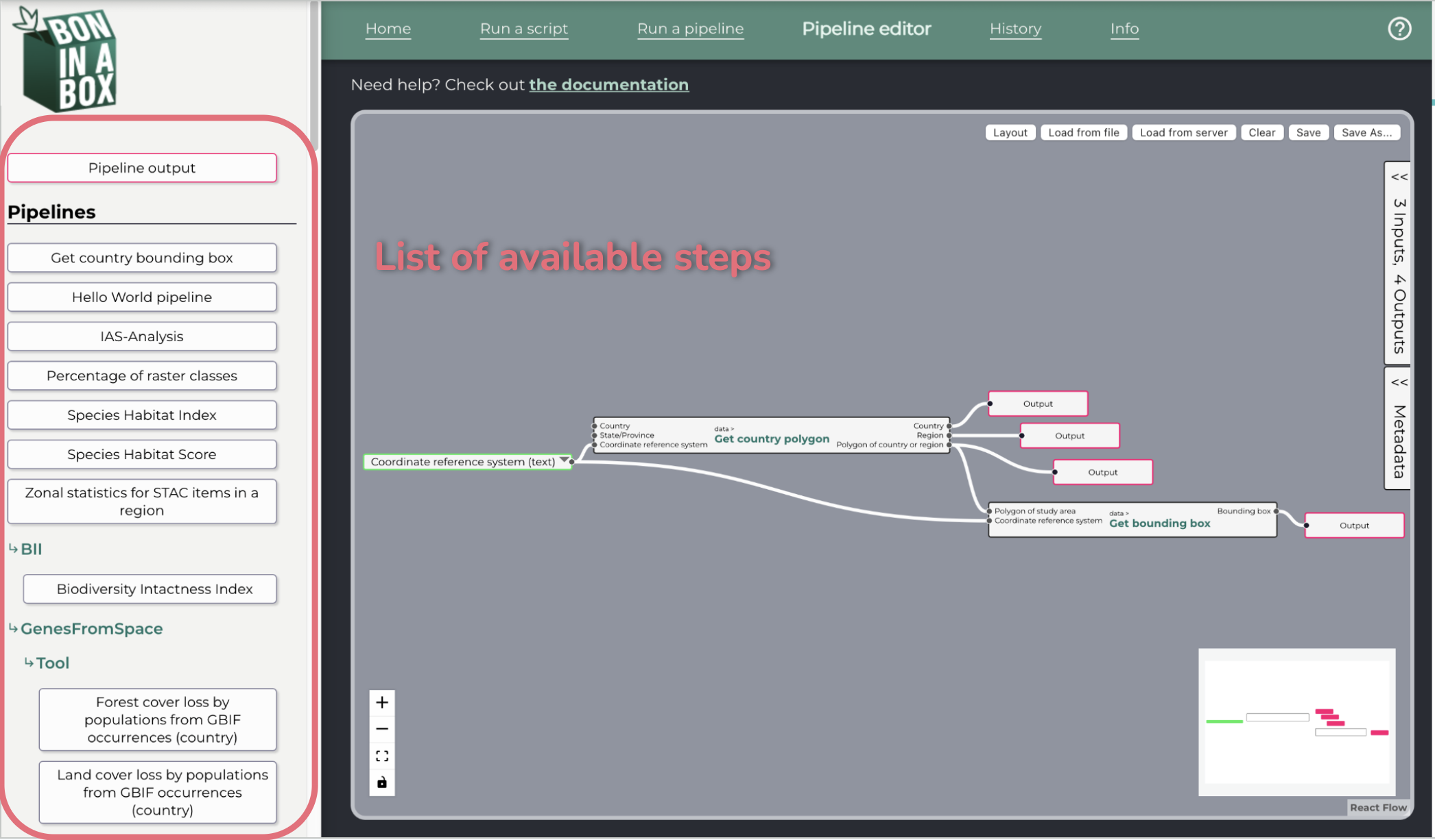
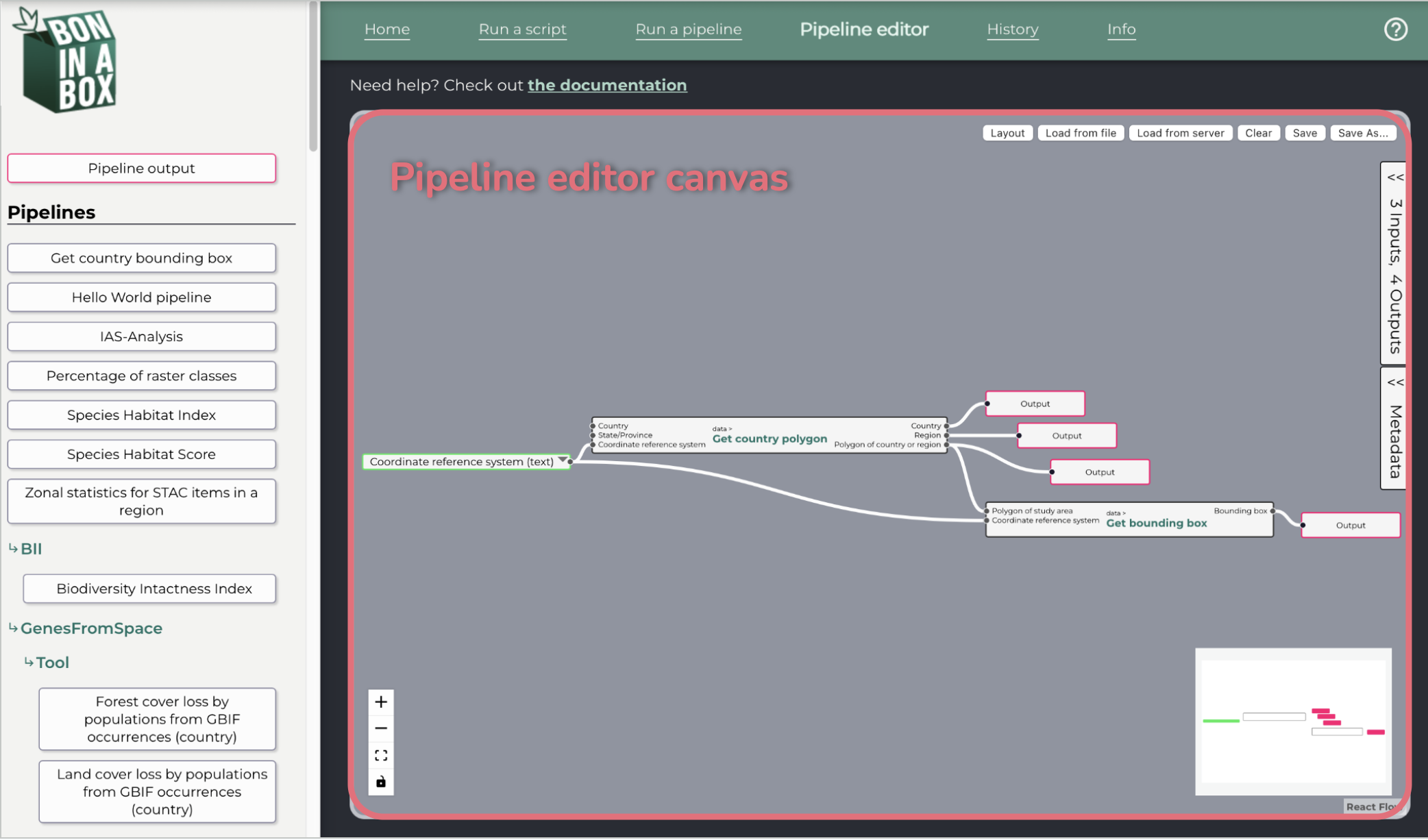
The pipeline editor allows the user to create pipelines by connecting individual scripts through inputs and outputs.
The left pane shows the available steps, which can be dragged onto the pipeline editor canvas.
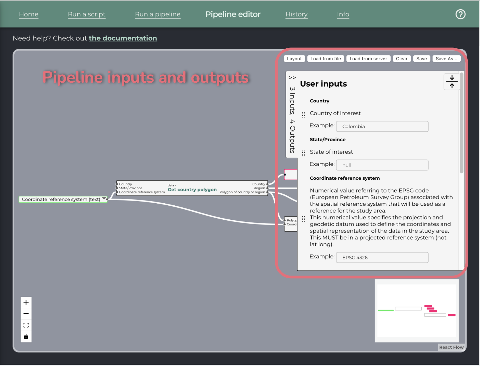
On the right side, a collapsible pane allows the user to edit the labels and descriptions of the pipeline inputs and outputs.
Below that pane, there is a pane for writing the metadata of the pipeline.
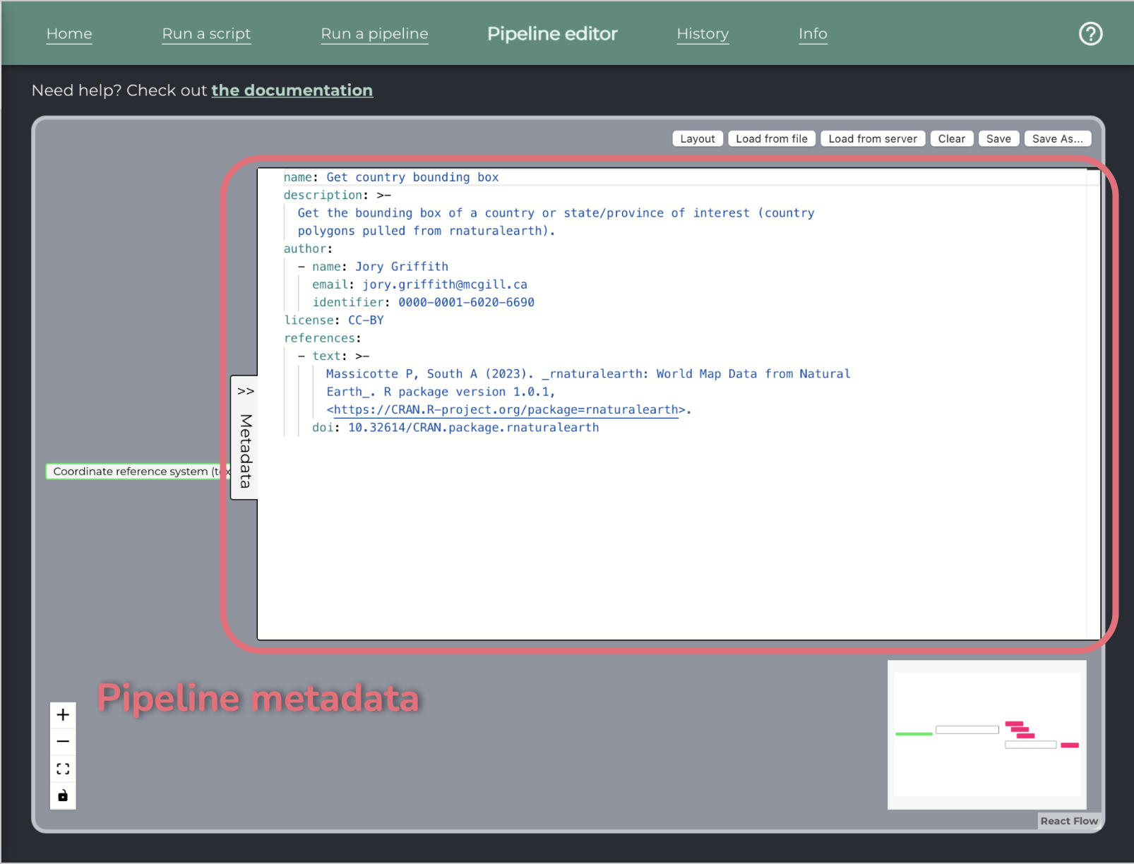
To add a step: drag and drop from the left pane to the canvas. Steps that are single scripts will display with a single border, while steps that are pipelines will display with a double border.
To connect steps: drag to connect an output and an input handle. Input handles are on the left, output handles are on the right.
To add a constant value: double-click on any input to add a constant value linked to this input. It is pre-filled with the example value.
To add an output: double-click on any step output to add a pipeline output linked to it, or drag and drop the red box from the left pane and link it manually.
To delete a step or a pipe: select it and press the Delete key on your keyboard.
To make an array out of single value outputs: if many outputs of the same type are connected to the same input, it will be received as an array by the script.

A single value can also be combined with an array of the same type, to produce a single array.

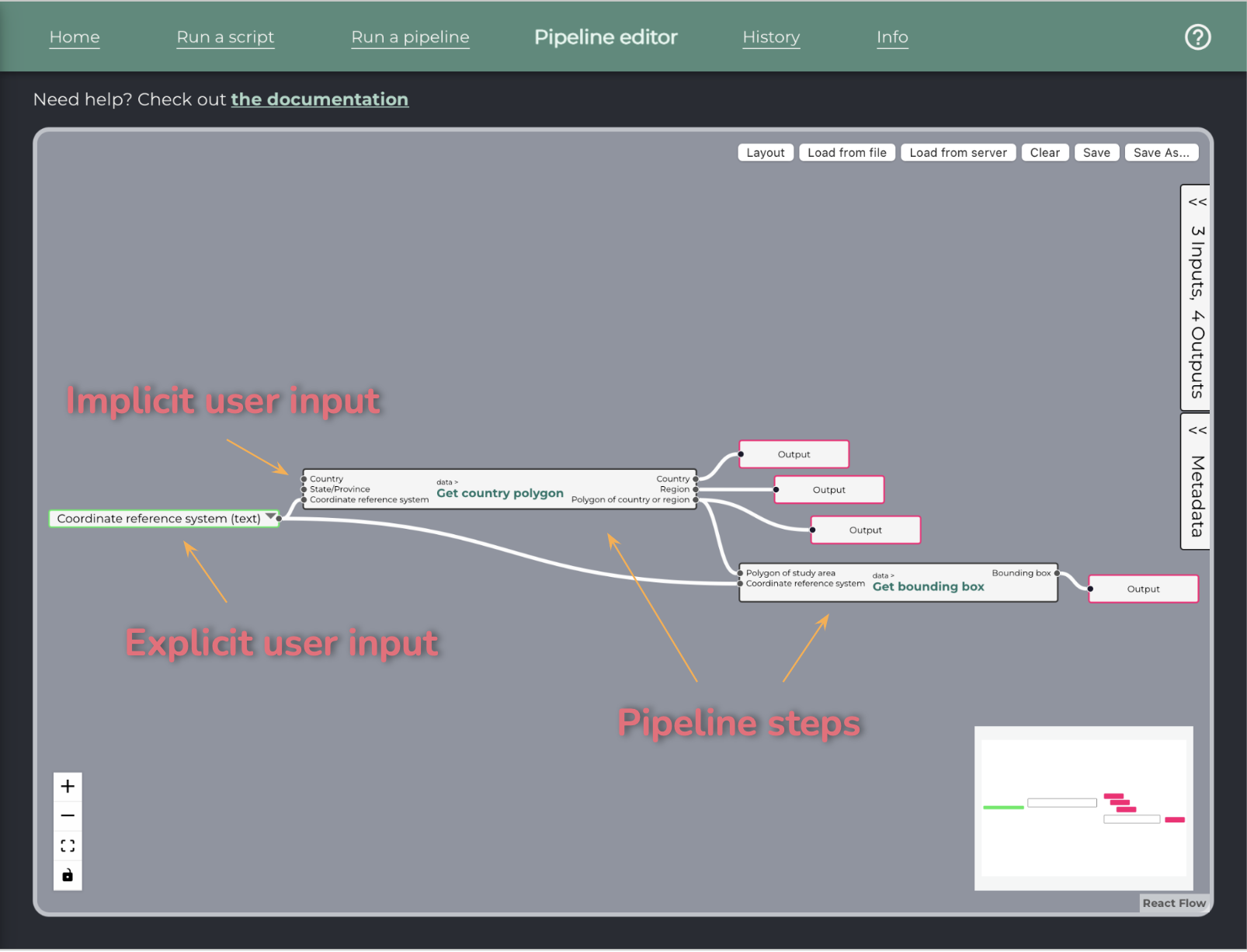
User inputs: To provide inputs at runtime, simply leave them unconnected in the pipeline editor. They will be added to the sample input file when running the pipeline.
If an input is common to many steps, a special user input node can be added to avoid duplication. First, link your nodes to a constant.

Then, use the down arrow to pop the node’s menu. Choose “Convert to user input”.

The node will change as shown below, and the details will appear on the right pane, along with the other user inputs.

Input type conversions
In most cases, an output can only receive a value of the exact same type. This means that if you plug an output of type “text/csv” to an input of type “float”, the system will display an error when saving the pipeline. However, there are exceptions where type conversions are allowed:
Source type |
Target type |
Example |
| Any type | An array of that type | When an array of GeoTIFFs is expected, a single GeoTIFF which is automatically wrapped in a single-element array.
|
| int | float | A buffer in kilometers received as an int by one script and as a float by another can share the same user input. 1 becomes 1.0 |
| options | text | A script receiving a link to any geospatial collection on a STAC as a string can be restricted at pipeline level to a few selected options. |
Pipeline inputs and outputs
Any input with no constant value assigned will be considered a pipeline input and the user will have to fill the value.
Add an output node linked to a step output to specify that this output is an output of the pipeline. All other unmarked step outputs will still be available as intermediate results in the UI.

Pipeline inputs and outputs then appear in a collapsible pane on the right of the canvas, where their descriptions and labels can be edited.
Once edited, make sure to save your work before leaving the page.
Saving and loading
The editor supports saving and loading on the server, unless explicitly disabled by host. This is done intuitively via the “Load from server” and “Save” buttons.
Step 7: Run pipeline and troubleshoot
The last step is to load your saved pipeline in BON and a Box and run it in the “run pipelines” tab.
Your pipeline should generate a form, which you can fill and then click run.
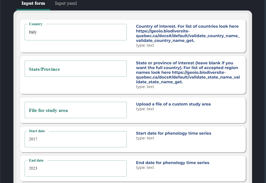
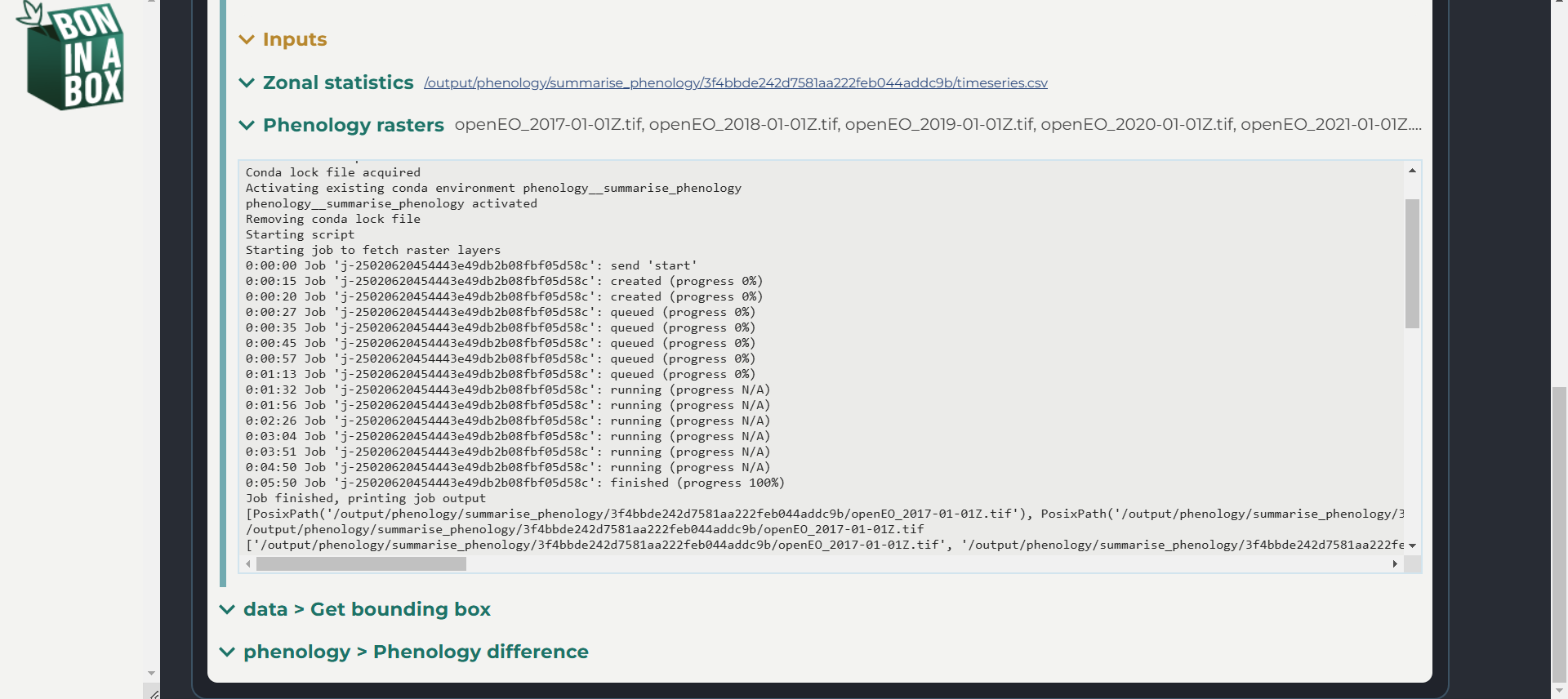
You can look at the log of each of your scripts to read errors and debug.
Once you change a script’s code and save to your local computer, the changes will immediately be implemented when you run the script through BON in a Box. However, if you change the YAML file, you will need to reload the page in the pipeline editor to see those changes. If this does not work, you may need to delete the script from the pipeline and re-drag it to the pipeline editor. Inputs and outputs can also be directly edited in the pipeline editor.
Troubleshooting
Here are some common issues when trying to run pipelines in BON in a Box and how to fix them.
The pipeline editor displays a warning when saving your pipeline
Errors in saving pipelines are usually due to incompatible inputs and outputs. When you change inputs or outputs in the script description’s YAML file, this won’t automatically change on the pipeline editor. When adding inputs, reload the pipeline editor so it reflects your changes. When changing the file formats of inputs or outputs, you will need to delete the edited script from the pipeline and re-drag it into the pipeline editor so that it can be saved. Note that pipelines saved with an error cannot be ran.
The script can’t find your packages
Make sure that all of packages available on anaconda.org are in the Conda sub-environment in the script description YAML file. If they are not on anaconda, install them via the regular installation mechanism of your programming language.
“Script produced no results.”
a. Check log for errors: the script might have crashed without leaving any error message for BON in a Box to display. If you are developing the script, detecting the preconditions for this crash and adding a call to
biab_error_stopbefore it crashes is recommended.b. Make sure that the script calls
biab_output: BON in a Box displays only the outputs that were specified using thebiab_outputfunction during the script’s execution. These outputs should have a corresponding definition in the script description yml file.c. Monitor the memory usage on next run: see memory section below.
Not enough memory (RAM)
The memory usage of BON in a Box alone is around 1GB. Then, depending on the analysis that is run, the scripts will take more memory. Normally, large datasets or large regions take more memory. That relation can be linear or exponential depending on the analysis.
Operating systems have programs that one can use to monitor the memory usage. Use the Task Manager on Windows, the Activity Monitor on a Mac, or for Linux use
htopor similar.
If you encounter further errors, please contact us on Discourse or email us at boninabox@geobon.org.
When is your pipeline complete?
The pipeline is generalizable (for example can be used with other species, in other regions)
The pipeline meets all of the standards in the quality control requirements
Each step has documentation for each input, output, references, etc. It should be easy enough to understand for a normal biologist (i.e. not a subject matter expert of this specific pipeline)
Each step validates its inputs for aberrations and its outputs for correctness. If an aberration is detected an “error” should be returned to halt the pipeline, or a “warning” to let it continue but alert the user.
The GitHub actions pass.
You have created a tutorial to go along with your pipeline, following [this template](https://github.com/GEO-BON/bon-in-a-box-pipelines/blob/main/pipelines/New-pipeline/pipeline-tutorial-template.md).